Predicting House Prices with Linear Regression: A Machine Learning Approach For Beginners

In this concise exploration of Machine Learning, we employ the California Housing dataset to predict house prices using a Linear Regression model implemented in a Jupyter Notebook. This model examines key features, like the average number of rooms per dwelling, to forecast prices effectively. Repository URL: house-price-prediction-model

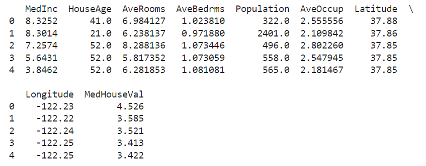
Dataset Exploration: Understanding the dataset's structure and key features.

Model Implementation: Utilizing scikit-learn to implement the Linear Regression model.

# Identify the feature variable(s) and target variable.
# In this case, we choose "AveRooms" (average number of rooms per dwelling) as feature and "MedHouseVal" as target.
X = pd.DataFrame(np.c_[data["AveRooms"]], columns=["AveRooms"])
Y = data["MedHouseVal"]

# Split our data into training and testing subsets.
X_train, X_test, Y_train, Y_test = train_test_split(
X, Y, test_size=0.2, random_state=9
)

# Define, fit, and run our linear regression model using train data.
model = LinearRegression()
model.fit(X_train, Y_train)

# Evaluate the model using the test data.
Y_pred = model.predict(X_test)

# Create metrics (like Mean Squared Error) to assess our model's performance.
mse = metrics.mean_squared_error(Y_test, Y_pred)
print("Mean Squared Error: ", mse)

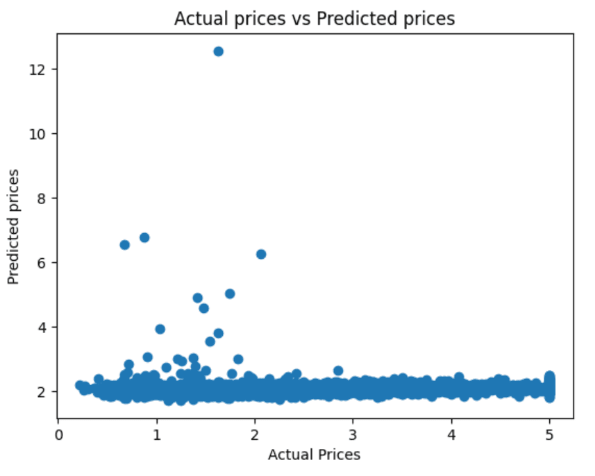
Model Evaluation: The model's predictions are plotted against the actual house prices, showing how closely the model's predictions align with reality. The Mean Squared Error for our model is 1.340961179318387, indicating the average squared difference between the estimated values and the actual value.

The project is thoroughly documented in a Jupyter Notebook, making it accessible for both beginners and experienced practitioners. This approach not only demonstrates the model's predictive capabilities but also highlights areas for improvement.